Glenn Chaple’s Observing Basics: Sketching 101

“But I can’t draw!”
It’s a complaint many an art teacher is all too familiar with. Perhaps you had the same thought upon discovering that our topic this month is astronomical sketching.

Sketching at the eyepiece isn’t as hard as you might think, as long as you don’t rush. Besides a telescope and eyepieces, you’ll need a clipboard, a sheet of paper with a circle on it to represent the field of view, and a few sharpened #2 pencils with erasers. You’ll also need a flashlight covered with red cellophane to preserve your night vision. Armed with these tools, you’re ready! Here’s how to create your own cosmic masterpiece.

Step 1
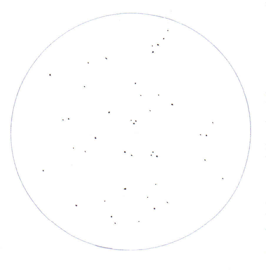
Center the subject (in this case, we’ll work with the Beehive Cluster [M44]) in the eyepiece’s field of view. Use a magnification that captures the entire cluster, as well as some of the surrounding space.
March 2010 Observing Basics sketches
Step 2
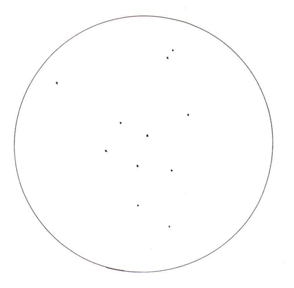
Begin by sketching “anchor” stars. These bright stars serve as reference points in your sketch. Carefully draw each star, noting its position in the field relative to the center and edge. It helps to think of the field edge as the face of a clock, with stars near the top marking the 12 o’clock position. Look for distinct star patterns like triangles or curved lines. As you add each star, note its position in relation to the ones already sketched. Because you’ll represent a star’s brightness by the size of the pencil dot you draw, make these dots fairly large and bold.
March 2010 Observing Basics sketches
Step 3
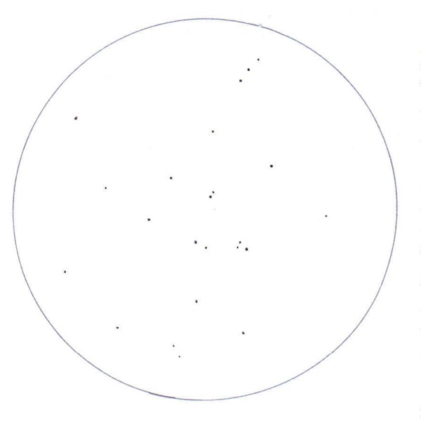
Add the fainter, but readily visible, member stars of the Beehive Cluster. Use the anchor stars to position them. Because you’re sketching fainter stars, the pencil dots should be less bold.
March 2010 Observing Basics sketches
Step 4
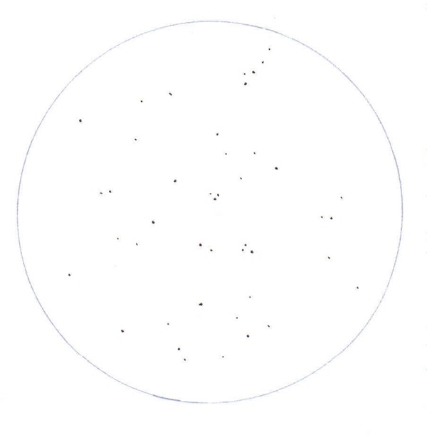
Here’s the part that hones your observing skills. Look carefully for faint stars that approach the limiting magnitude of your telescope (averted vision helps here). Represent each with tiny pinpoints.

Sketching may not be as fast and accurate as digital photography, but it forces you to take a good long look at your subject. You pick out subtle nuances you might miss with a casual glance.

Step 5
Your masterpiece is complete! All it needs is a title (in this case, “M44”), the date and time, the telescope you used, the eyepiece’s magnifying power, and sky conditions.

Questions, comments, or suggestions? E-mail me at gchaple@hotmail.com. Next month: A funny thing happened on the way to the observatory. Clear skies!


Learn more sketching techniques
For further information on astronomical sketching, be sure to follow David J. Eicher’s “Deep-sky Showcase” in each issue of Astronomy (page 68 this month). You can observe the objects he suggests and compare sketching results.

For more Internet resources, log on to Bill Greer’s astronomy site at www.rangeweb.net/~sketcher. In addition, look into Math Heijen’s how-to at www.backyard-astro.com/focusonarchive/sketching/sketching.html. For a video clip featuring Dave Eicher, subscribers can visit www.Astronomy.com/videos. Click on “How to,” and scroll down toward the bottom to get to “Sketching from the telescope.”

Finally, from Patrick Moore’s Practical Astronomy Series comes an excellent book, Astronomical Sketching (Springer, 2007). You’ll find in-depth instruction on a variety of astro-sketching techniques from authors Richard Handy, David B. Moody, Jeremy Perez, Erika Rix, and Sol Robbins.


Read more of Glenn Chaple’s Observing Basics
February 2010: Astroimaging 101
See an archive of Glenn Chaple’s Observing Basics

SwRI researchers offer explanation for the differences between Ganymede and Callisto

Jupiter and moons
Jupiter (right) and the Galilean satellites (right to left) Io, Europa, Ganymede, and Callisto. Cutaways show the interior states of Ganymede and Callisto after many impacts by icy planetesimals during the Late Heavy Bombardment. Colors represent density, with black showing the rocky core (with a density 3 g/cm^3), blue showing mixed ice and rock (densities 1.8 to 1.9 g/cm^3) and white showing rock-free ice.
SwRI, San Antonio, Texas
January 25, 2010
Differences in the number and speed of cometary impacts onto Jupiter’s large moons Ganymede and Callisto some 3.8 billion years ago can explain their vastly different surfaces and interior states, according to research by scientists at the Southwest Research Institute (SwRI) in San Antonio, Texas.

Ganymede and Callisto are similar in size and are made of a similar mixture of ice and rock, but data from the Galileo and Voyager spacecraft show that they look different at the surface and on the inside. A conclusive explanation for the differences between Ganymede and Callisto has eluded scientists since the Voyager-Jupiter encounters 30 years ago.

Amy C. Barr and Robin M. Canup of the SwRI Planetary Science Directorate created a model of melting by cometary impacts and rock core formation to show that Ganymede’s and Callisto’s evolutionary paths diverged about 3.8 billion years ago during the Late Heavy Bombardment, the phase in lunar history dominated by large impact events.

“Impacts during this period melted Ganymede so thoroughly and deeply that the heat could not be quickly removed,” said Barr. “All of Ganymede’s rock sank to its center the same way that all the chocolate chips sink to the bottom of a melted carton of ice cream. Callisto received fewer impacts at lower velocities and avoided complete melting.”

In the Barr and Canup model, Jupiter’s strong gravity focuses cometary impactors onto Ganymede and Callisto. Each impact onto Ganymede or Callisto’s mixed ice and rock surface creates a pool of liquid water, allowing rock in the melt pool to sink to the moon’s center. Ganymede is closer to Jupiter and therefore is hit by twice as many icy impactors as Callisto, and the impactors hitting Ganymede have a higher average velocity. Modeling by Barr and Canup shows that core formation begun during the Late Heavy Bombardment becomes energetically self-sustaining in Ganymede but not Callisto.

The study sheds new light on the “Ganymede-Callisto dichotomy,” a classical problem in comparative planetology, a field of study that seeks to explain why some solar system objects with similar bulk characteristics have radically different appearances. In particular, the study links the evolution of Jupiter’s moons to the orbital migration of the outer planets and the bombardment history of Earth’s Moon.

“Similar to Earth and Venus, Ganymede and Callisto are twins, and understanding how they were born the same and grew up to be so different is of tremendous interest to planetary scientists,” said Barr. “Our study shows that Ganymede and Callisto record the fingerprints of the early evolution of the solar system, which is very exciting and not at all expected.”

The multiverse: Why do other universes not collide with ours?

Our observable universe is the region of space that we can see today — all points in space in which the light has had enough time to reach us if it left those points at the Big Bang (13.7 billion years ago) or later. The multiverse consists of our observable universe and all of space outside of it — so, everything that is “out there.”

One of the most common meanings of “other universes” is “bubble universes” predicted by cosmological inflationary theory. They are regions of space where inflation was particularly successful, and these regions grow extremely fast. These bubble universes may have observers much like ours, and typically they are at great distances from us (much larger than the radius of our observable universe, which is about 50 billion light-years).

Any future collision between our observable universe and a bubble universe will presumably happen on cosmological timescales — tens of billions of years or longer. So we shouldn’t expect a collision to happen next month. In fact, we hope it won’t because the collision would progress with the speed of light and destroy our habitat at the same instant we would see it.

However, it is also possible that our observable universe collided with another bubble universe in the past. If that’s the case, the cosmic microwave background (CMB) radiation may well hold relics of such a collision. Predicting the form of these relics and searching for them in the CMB is an area of current research. — Dragan Huterer, University of Michigan, Ann Arbor

Saturn’s rings reappear

March 2010 saturn rings
Saturn’s rings tilt 3° to our line of sight at this month’s opposition, slightly more than in this Hubble Space Telescope view from February 2009. Notice orange Titan and its black shadow crossing Saturn’s north polar region.
NASA/ESA/Hubble Heritage Team (STScI/AURA)

The March skies open with a spectacularly bright Venus hugging the western horizon just after sunset. Late in the month, Mercury joins Venus in the evening twilight. Mars rides high in the southeast as darkness falls. Although it is now past its best, the Red Planet remains an attractive sight with naked eyes and a worthwhile target for those with medium-sized scopes.

5 more astronomy questions

March 2010 WE Epsilon Eridani
Astronomers have found more than 400 planets beyond our solar system. The nearest one known lies 10.5 light-years away and orbits the star Epsilon Eridani. In this illustration, a hypothetical family of moons orbits the planet.
NASA/ESA/G. Bacon (STScI)

In Astronomy’s March 2010 issue, I shared insight into five of the biggest questions facing astronomy today. But that was just an arbitrary list, and there are plenty more cosmic conundrums scientists face every day. So below I address five more questions that have crossed many minds over the years.

The story of a variable star observation

January 22, 2010
The American Association of Variable Star Observers (AAVSO) is the world’s largest organization dedicated to observing and studying variable stars. Headquartered in Cambridge, Massachusetts, the AAVSO boasts more than 2,500 members and contributing observers from more than 55 countries. These dedicated individuals monitor the brightness of variable stars visually or with charge-coupled devices and forward the information to the AAVSO database, where it is made available to astronomers around the world. Since its formation in 1911, the AAVSO has received 17 million variable star estimates. Here’s the story of just one.

Selecting a star
I begin by logging on to the AAVSO website at www.aavso.org. Scrolling down the menu on the left side of the homepage, I arrive at “Variable Stars,” which, in turn, leads me to a section titled “Stars Easy-to-observe.”

From the list of easily observable stars, I select the Mira-type variable T Cassiopeiae. It’s currently visible in the evening sky, and its magnitude range (6.9-13.0 over a 445-day cycle) is within the grasp of my 10-inch reflector.

Making a chart
To estimate T Cas’ brightness, I’ll need a chart showing the variable and nearby comparison stars — field stars whose magnitudes are noted. A few decades ago, this meant filling out a chart request form and mailing it, along with the appropriate amount of money, to AAVSO Headquarters in Cambridge. After about a week, the chart would arrive in the mail.

How times have changed! Returning to the menu on the left side of the AAVSO home page, I scroll down to “Make a Chart.” This brings me to a form (AAVSO Variable Star Plotter — VSP, for short) that allows me to tailor-make charts. Following the prompts, I generate and print out three charts: a 15°-wide “A” scale chart that includes enough of Cassiopeia’s main stars to help me locate T Cas; a “B” scale chart whose 3° field and 11th-magnitude limit allows me to study T Cas when it is at its brightest; and a 0.5° “E” scale chart set for a limiting magnitude of 14 for times when T Cas is near minimum. What used to take a week now requires less than 10 minutes — and it’s free!

Making and recording a brightness estimate
Here’s where the fun begins! Using the “A” chart, I aim my telescope toward a bright star in Cassiopeia (Zeta [ζ] Cas). Switching to the “B” chart, I star-hop from Zeta to T Cas. T Cas lies beside an 8.1 magnitude comparison star (labeled “81” on the chart — decimals are omitted so they won’t be mistaken for field stars). Because T Cas is noticeably fainter than its magnitude 8.1 neighbor, I scan the field for a fainter comp star. One labeled “88” appears to be equal in magnitude to T Cas, and a magnitude 9.2 field star is slightly fainter. After careful scrutiny, I decide that T Cas and the 8.8 mag star are essentially equal in brightness. On a data sheet, I record the date and time of my observation (in Julian date form), the star name, its magnitude, and the magnitudes of the comparison stars.

Sending the data to AAVSO Headquarters
Three decades ago, I would save all my data sheets until month’s end when I’d transpose all variable-star estimates (often numbering in the hundreds) onto AAVSO observing forms. The process often took hours to complete. The Internet makes things quicker, easier, and (most importantly) timelier.

After observing T Cas, I return home, turn on the computer, and log on to the AAVSO home page. Scrolling down the left side menu, I select “Web Obs.” After entering my AAVSO username and password, I see a page that allows me to submit my T Cas information to the AAVSO database. The entire process takes less than a minute. The AAVSO gets the data immediately, not at the end of the month.

A final step — instant gratification!
Mission accomplished! Now, I’d like some idea of the accuracy of my observation. Years ago, I knew a few AAVSO members who encouraged me to mail them my variable star estimates, after which they’d write back and let me know how mine compared with theirs. Not exactly the best way to get timely verification! Fortunately, the Internet has changed that.

Seconds after submitting my data on T Cas, I return to the AAVSO home page and select “Quick Look” on the menu. The Quick Look request form appears on the screen, and I type in the star name and click on the “Search” prompt. This results in a chronological listing of magnitude estimates of T Cas submitted by AAVSO observers. Previous estimates of T Cas agree closely with mine. My observation is validated!

I’m not done! Once more, I return to the AAVSO homepage, this time selecting “Light Curve Generator.” This produces a graph (the light curve) that combines all of the observations submitted for a particular variable star over a specific time period — a dramatic visual display of its recent behavior. Within seconds of typing in the star name and selecting a time increment (I choose the past 500 days — a little longer than T Cas’ period), its light curve appears on the screen. A sine-like wave, composed of hundreds of dots, shows the rise and fall of T Cas through a complete cycle. Each of those dots represents another AAVSO observer’s data. Mine, being the most recent, lies at the graph’s far right. Like a solitary note from a musician, that one single observation, combined with those of dozens of other AAVSO members, has formed this beautiful symphony of a light curve!

And that, my friend, is the story of a single variable star estimate.

National Science Foundation selects National Solar Observatory to build world’s largest solar telescope

The Sun
Double prominences.
SOHO/ESA/NASA
January 22, 2010
The National Science Foundation has awarded a $298 million cooperative support agreement to the Association of Universities for Research in Astronomy (AURA) to build the 4-meter Advanced Technology Solar Telescope (ATST).

“I want to congratulate everyone who has helped make this happen,” said Stephen L. Keil, director of the National Solar Observatory (NSO) and AURA’s principal investigator for ATST. “It should be an exciting next several years as we bring ATST to reality.”

ATST will be the largest and most capable solar telescope. No comparable facility exists or is planned. ATST will be the world’s flagship facility for the study of magnetic phenomena in the solar atmosphere and will be the first large, ground-based, open-access solar telescope in the United States in more than 40 years.

“This is an exciting opportunity for the NSO to lead the community,” said William Smith, president of AURA. “We look forward to achieving a first-rate, cutting-edge facility.”

ATST is to be built atop Haleakala, Maui, Hawaii, pending completion of a Conservation District Use Agreement and other permits. Haleakala was selected after considering 72 sites and then narrowing those down to six for additional consideration through on-site testing. Of those six sites, only the Haleakala site met all of ATST’s requirements — the least atmospheric blurring, the most annual hours of low sky brightness, the lowest dust levels, and the smallest temperature extremes. The site is next to the existing Mees Solar Observatory that is owned and operated by the University of Hawaii’s Institute for Astronomy, a principal partner in the project.

Understanding the role of magnetic fields in the outer regions of the Sun is crucial to understanding the solar dynamo, solar variability, and solar activity, including flares and mass ejections, which can significantly affect life on Earth. ATST research will investigate solar variability and its impact on terrestrial climate — the conditions responsible for solar flares, coronal mass ejections, and other activities that can impact terrestrial communications and power systems, disrupt satellite communications, and endanger astronauts and air travelers.

ATST’s 4-meter primary mirror will feed an advanced array of instruments designed to study the Sun in light ranging from near ultraviolet (350 nm) into the far infrared (28,000 nm, or 28 microns). High-order adaptive optics, pioneered by the NSO and its partners at NSO’s Dunn Solar Telescope at Sunspot, New Mexico, will correct blurring of solar images caused by Earth’s atmosphere, thus allowing ATST to observe features in the solar atmosphere with unprecedented sharpness, down to structures only a few tens of kilometers in size.

ATST will observe both on the bright solar disk and in the ultra-faint corona. ATST will accurately measure magnetic fields in the ultra-faint corona, which is only a few parts in a million as bright as the solar disk.

NASA reveals new batch of space program artifacts

NASA artifacts
Potential artifact: Mockup suit [Mercury].
NASA/JPL-Caltech/University of Arizona
January 22, 2010
NASA is inviting eligible education institutions, museums, and other organizations to examine and request space program artifacts online. The items represent significant human space flight technologies, processes, and accomplishments from NASA’s past and present space exploration programs.

NASA partnered with the General Services Administration (GSA) to provide a first-of-its-kind, Web-based, electronic artifacts prescreening capability last year. On October 1, 2009, the GSA launched a Web initiative for screening and requesting NASA’s space shuttle artifacts. The first round ended November 30, and all 913 artifacts were allocated.

A second Web-based screening opportunity began January 19. It includes approximately 2,500 potential artifacts from NASA programs that include the space shuttle, Hubble Space Telescope, Apollo, Mercury, and Gemini. It is available at gsaxcess.gov/NASAWel.htm. Each artifact will be screened for 90 days. After the screening period closes, and at the completion of the allocation process, requestors will be notified about the status of their request.

Museums and schools will be screened for eligibility through an online registration process or through their state agency for surplus property. Eligible recipients may view the available artifacts and request specific items at the Web site. Prescreening allows potential recipients to identify specific items and provides the time to plan to transport, preserve, and properly display artifacts.

Requesting an artifact through the prescreening process does not guarantee the item will be available. Nor does it provide a specific time when it will become available. Allocated artifacts will be incrementally released as they are no longer needed by NASA and in accordance with export control laws and regulations.

Although the artifacts are provided without charge, eligible recipients must cover shipping and any special handling costs. Shipping fees on smaller items will be relatively inexpensive, while larger items may involve extensive disassembly, preparation, shipping, and reassembly costs. NASA will work closely with potential recipients on a case-by-case basis to address any unique special handling costs.