When rejection is good, part 1

The genesis for this column comes from my experience with image processing. When I began digital photography in the early 1990s, most amateurs would take pictures totaling a few minutes of exposure and add them together. These grayscale images far exceeded what could be accomplished with film in the same period of time.

More experienced imagers combined RGB-filtered images. However, the exposure times and number of frames collected remained small. Interestingly, imagers often would buy larger instruments and more sensitive cameras before increasing the exposure duration and number.

Later, the seemingly esoteric practices of image processing, done by professional astronomers, trickled down to the amateur realm through the inclusion of utilities in popular software. One such area is the statistical analysis of data, which permits the identification and management of unwanted sources of noise and signals. Before imaging software included these tools, it was extremely difficult to eliminate satellite trails, defects on chips, and cosmic rays.

When I accommodated visitors at Kitt Peak National Observatory as part of an observing program I developed that ran from 1996 to 2005, I spent countless hours manually removing these “vermin” from pictures while guests often fell asleep behind me. After all, guests expected to go home with pretty pictures by the end of a night! As I used Photo-shop’s “Clone” tool (and later the “Healing” brush), visitors often would be concerned that I might erase a galaxy rather than a cosmic ray.

Nowadays, guests who visit me at the Mount Lemmon SkyCenter have a much better experience joining me in the processing of images. The tedium of removing cosmic rays is a thing of the past. In order to understand how this happened, you must understand the nature of light and the power of statistics. Every time we take an exposure, each pixel of the detector is making a measurement. When I take a 20-minute exposure, the picture that results has a single value for each pixel.

Because of the particle nature of light, the number of photons a CCD chip detects fluctuates with each exposure. If the average intensity of a star on a specific pixel is 1,000 counts (brightness units), then in the first exposure I might measure 943 counts, and in the next exposure it may be 1,078 counts. So, if I take enough exposures and average them together, the resulting value will be a good approximation of the intensity. Unfortunately, we never know what this average value should be beforehand. That’s why we need to make many measurements to find the average (or mean) value.

Image #1 graphically shows an analog to these fluctuations. In Photoshop, I took a simple column of six pixels that display a low-contrast pattern (a mere two shades of gray) and applied “Add Noise” to imitate fluctuations. After generating 11 pseudo-measurements, I then created the column labeled “Average.” Note that you would be hard-pressed to identify the expected pattern from any individual row. Only after averaging the results does it start to approximate the “Ideal” form.

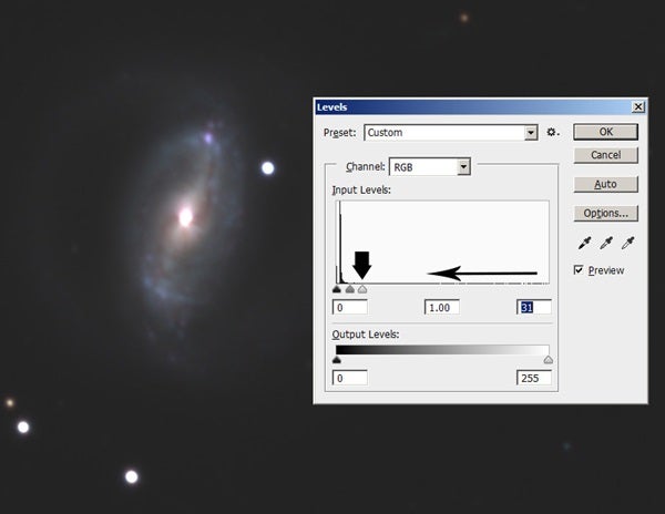
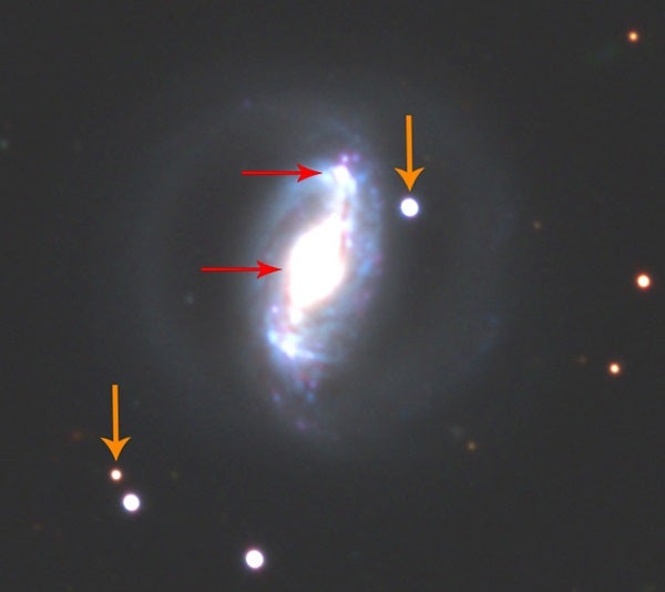
Image #2 shows a real-world example. The left side is a single measurement, and the right half is the average of 20 values at each pixel for a strange planetary nebula called WeBo 1. Closer inspection shows some bright blips in the single exposure that are not in the average image. Most of these are cosmic rays, which represent values we do not want to include when calculating the mean of a set of measurements.

In Image #3, a cosmic ray (a white pixel) was part of the fifth measurement. It contaminated the resulting mean value for that pixel, and it degrades the image quality. What we want to do is identify such outlying values and not use them when calculating the mean.

This means that for the 20 values measured at a particular pixel in the WeBo 1 image, if a cosmic ray activated that pixel, we should reject that value and calculate the mean from the remaining 19 values. This greatly improves the image quality and eliminates transient signals in our images.

In my next column, we will look at how to measure the average amount of fluctuation and then identify these outlying values.